
PCA Explained Simply: Understanding Dimensionality Reduction

In our previous article on unsupervised learning, we covered a clustering algorithm. Today we will be covering a common algorithm that comes under the category of dimensionality reduction.
So, in machine learning, having more data is usually helpful but having too many features can sometimes create more problems than benefits. High-dimensional data can slow down algorithms, increase memory usage, cause overfitting, and make visualization nearly impossible. This is where dimensionality reduction comes in, and one of the most widely used techniques for this purpose is Principal Component Analysis (PCA).
PCA is an unsupervised learning technique that reduces the number of features in a dataset while preserving as much important information as possible. Instead of selecting existing features, PCA creates new features, called principal components, which summarize the original data in a more compact form.
What Is PCA (Principal Component Analysis)?
Principal Component Analysis is a technique that transforms a dataset with many correlated features into a smaller set of uncorrelated components. These components capture the directions where the data varies the most. In simple terms, PCA helps remove redundancy from data and keeps only what matters the most.
Think of a dataset with features like age, salary, years of experience, and monthly income. Many of these features are related to each other. PCA identifies these relationships and combines them into fewer dimensions without losing the overall structure of the data.
Intuition Behind PCA (Simple Explanation)

Imagine a cloud of data points floating in space, like stars in the sky. If you look at this cloud from the wrong angle, it may look scattered and confusing. But if you rotate your view to the right angle, you’ll notice clear patterns and structure.
Imagine you are taking a group photo of many people standing close together. From some angles, the photo looks messy and crowded, but from the right angle, you can clearly see everyone. PCA finds these best angles automatically.
In another way, think of students described by height, arm length, and leg length. These features are strongly related. PCA combines them into a smaller number of components representing overall body size, reducing complexity without losing essential information.
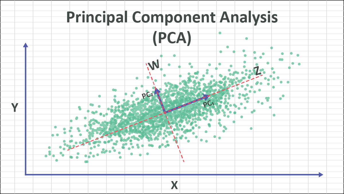
PCA finds these best viewing angles automatically. These angles are called principal components.
The first principal component captures the maximum variance in the data (where data is spread out the most). The second principal component captures the next highest variance, but in a direction orthogonal (perpendicular) to the first. This process continues until all dimensions are covered.
Why Do We Need PCA?
PCA is mainly used to simplify complex datasets while keeping the most important information intact. It helps reduce noise, remove redundancy, and improve computational efficiency. Many machine learning algorithms perform better when trained on fewer, meaningful features rather than a large number of correlated ones.
PCA is especially useful when:
The dataset has many features
Features are highly correlated
Visualization is difficult due to high dimensions
Models are slow or overfitting
How PCA Works (Step-by-Step)
PCA follows a structured mathematical process.
First, the data is standardized so all features are on the same scale. This is necessary because PCA is sensitive to feature magnitude.
Next, PCA computes the covariance matrix, which shows how features vary with respect to each other. This helps identify correlated features.
Then, PCA finds principal components, which are new axes where the data has the highest variance. The first principal component captures the maximum variance, the second captures the remaining variance while being orthogonal to the first, and so on.
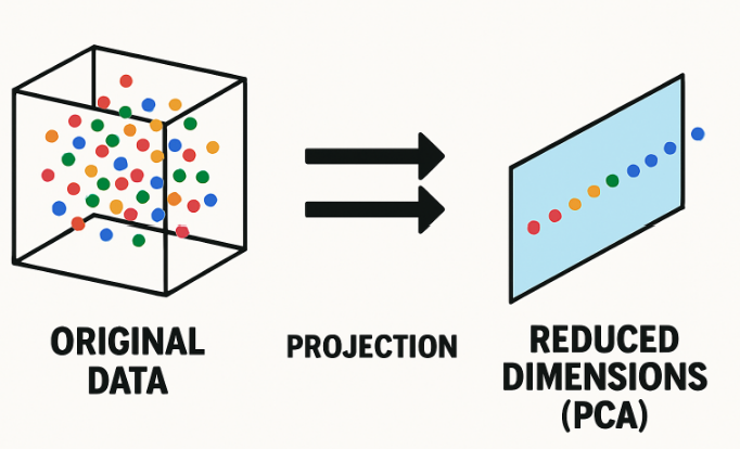
Finally, the data is projected onto the top K principal components, reducing dimensionality while preserving most of the information.
Key Concept: Variance and Information
The main goal of PCA is to maximize variance. Variance represents information in the data. The more variance a component captures, the more information it retains from the original dataset.
The first principal component captures the most variance. The second captures the remaining variance while being uncorrelated with the first, and so on. In practice, just the first few components often capture 80–95% of the total variance, which is why PCA is so effective.
PCA & Feature Selection
PCA and feature selection both reduce dimensionality, but they work differently. Feature selection keeps a subset of the original features, preserving their meaning and interpretability. PCA, on the other hand, creates new features by combining existing ones, which improves efficiency but reduces interpretability. PCA is best when performance matters more than understanding individual features.
Real-World Applications of PCA
PCA is widely used both as a standalone technique and as a preprocessing step before applying machine learning models.
It is commonly used to visualize high-dimensional data by reducing it to 2D or 3D.
It helps in data compression, reducing storage and computation costs.
In business analytics, PCA simplifies complex datasets to support better decision-making.
In machine learning pipelines, PCA improves performance by reducing noise and overfitting.
Assumptions and Limitations of PCA
Although PCA is powerful, it comes with certain assumptions and limitations. PCA assumes that features are linearly correlated. If features are unrelated, PCA cannot find meaningful components.
PCA is also sensitive to feature scale, which is why standardization is mandatory. It is not robust to outliers, as extreme values can significantly affect variance. Additionally, PCA assumes linear relationships, so it cannot capture complex non-linear patterns. Lastly, PCA usually requires datasets without missing values.
Practical Implementation ( Wine Dataset)
Goal is to
Reduce 13 features → 2 principal components
Visualize high-dimensional data
Understand variance preservation
# Import libraries
import matplotlib.pyplot as plt
from sklearn.datasets import load_wine
from sklearn.preprocessing import StandardScaler
from sklearn.decomposition import PCA

# Load dataset
wine = load_wine()
X = wine.data   # only features (unlabeled data)

# Standardize features
scaler = StandardScaler()
X_scaled = scaler.fit_transform(X)


# Apply PCA (reduce to 2 dimensions)
pca = PCA(n_components=2)
X_pca = pca.fit_transform(X_scaled)

print("Explained variance ratio:", pca.explained_variance_ratio_)
print("Total variance captured:", sum(pca.explained_variance_ratio_))

plt.figure(figsize=(8, 6))
plt.scatter(X_pca[:, 0], X_pca[:, 1], s=50)
plt.xlabel("Principal Component 1")
plt.ylabel("Principal Component 2")
plt.title("PCA: Data Reduced from 13D to 2D")
plt.grid(True)
plt.show()

This plot shows the original 13-dimensional dataset compressed into 2 principal components, making it easy to visualize. The explained variance (~55%) means these two components capture more than half of the important information in the data.
Even after reduction, the structure and patterns of the data are preserved, which is exactly the goal of PCA.
Final Thoughts
Principal Component Analysis is one of the most intuitive and widely used dimensionality reduction techniques in machine learning. It helps transform complex, high-dimensional data into a simpler and more meaningful form without losing important information. While PCA is not suitable for every problem, it is an essential tool to understand for anyone working with real-world data.
In the context of unsupervised learning, PCA completes the core 80/20 toolkit along with K-Means and DBSCAN, making it a powerful next step in your learning journey.
Follow us for more : ML Diaries by Fahd


